A team wins 3-0. You check the expected goals afterwards and discover Team A had 0.9 xG and Team B had 1.7 xG.
So who actually played better? The scoreboard gives one answer, but expected goals gives another.
This is where football analysis can become confusing. Actual goals determine who wins the match, and nothing will ever change that.
But when you are trying to predict what happens next, the final score does not always tell the complete story. A team can score three times from three difficult chances.
Another can create five excellent opportunities and somehow score none. Over a single match, finishing, goalkeeping and luck can produce enormous differences between goals and expected goals.
That is why xG has become so widely used in football analysis. The best approach, however, is not to choose one and ignore the other.
Actual goals tell you what happened. Expected goals help explain how it happened.
For future football predictions, you usually need both.
What Does Expected Goals Actually Measure?
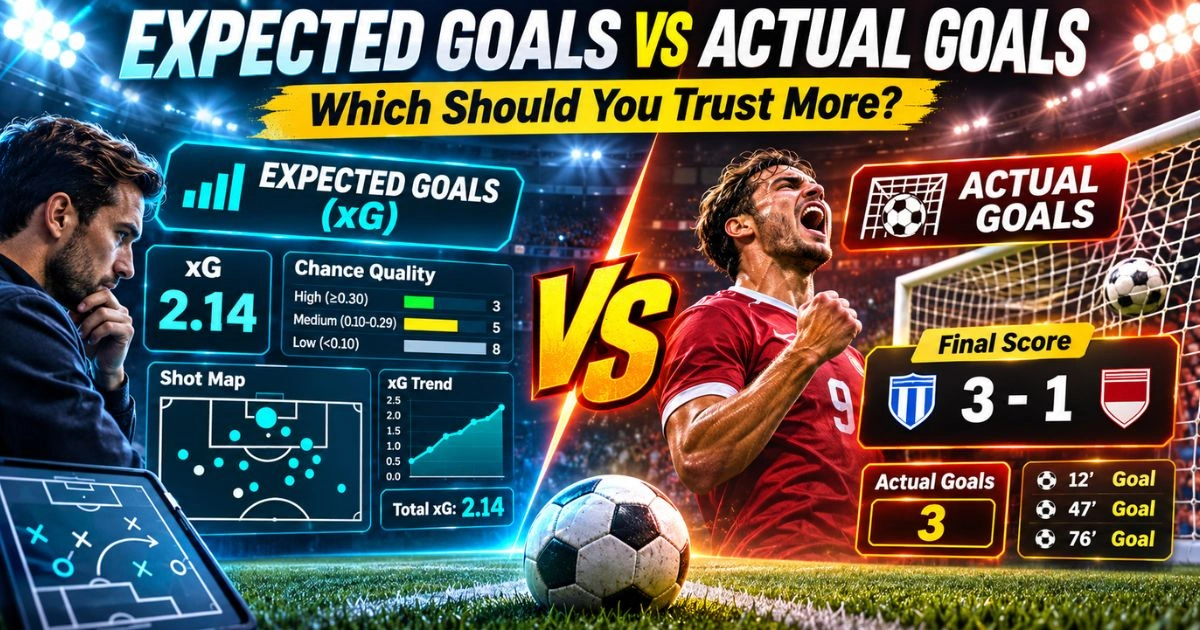
Expected goals—or xG—estimates the probability that a shot will become a goal based on similar historical attempts.Opta’s model uses information from nearly one million historical shots and scores chances between zero and one.
For example:
0.05 xG = roughly a 5% historical scoring probability
0.20 xG = roughly 20%
0.60 xG = roughly 60%
Opta’s model considers more than 20 variables, including shot distance, angle, goalkeeper position, defensive pressure, shot type and the action that created the opportunity. A penalty, for example, is valued at approximately 0.79 xG in Opta’s model because penalties have historically been converted around 79% of the time.
Actual Goals Measure Something Completely Different
Actual goals require no model. If the ball crosses the line legally, it is a goal.
A team scoring three times has three goals regardless of whether those shots had 0.1 xG or 0.8 xG. That makes actual goals perfect for measuring outcomes.
League tables are decided by real goals, and betting markets settle on real goals. Nobody receives points because they “won the xG.”
But that does not necessarily make actual goals the best statistic for predicting future performances.
Why Final Scores Can Mislead
Football is a relatively low-scoring sport. That means one unusual event can heavily influence the final score.
Consider this match:Team A
8 shots
0.7 xG
2 goals
Team B
17 shots
6 shots on target
2.1 xG
0 goals
Final score: Team A 2-0 Team B. If you analyse only the result, Team A looks comfortably superior.
But the underlying performance suggests something very different. Team B repeatedly created better opportunities but failed to finish them.
If these teams played ten more times under similar conditions, blindly assuming Team A would keep winning 2-0 would be dangerous.
Research Suggests xG Can Be More Predictive
This is one of the strongest arguments for expected goals. A 2023 peer-reviewed study compared xG with traditional statistics such as goals and shots across multiple leagues.
When the researchers examined how well current performance predicted goals in subsequent matches, expected goals generally outperformed actual goals and traditional shot statistics. Across the leagues studied, xG was superior in almost all of the prediction measures tested.
That does not mean xG predicts every match correctly. It means chance quality can provide a more stable picture of underlying team performance than recent finishing alone.
Practical Example: A Winning Team You Should Be Careful With
Imagine Team A’s last five matches:
Won 3-0
Won 2-0
Won 2-1
Won 1-0
Won 3-1
Total: 11 goals scored. Excellent form.
But its total xG during those matches is only 6.3. The team has scored 4.7 goals above xG.
That could mean several things. Perhaps Team A has elite finishers, faced weak goalkeepers, or several low-probability shots went in.
Or perhaps it is simply experiencing an unusually efficient period. You should not automatically predict another two or three goals simply because the recent scoreboard looks spectacular.
Practical Example: A Losing Team That May Be Better Than It Looks
Now imagine Team B’s last five:
Lost 0-1
Drew 1-1
Lost 0-2
Won 2-0
Lost 1-2
Only 4 goals scored. But Team B generated 8.1 xG.
That means the attack has created much better chances than its scoring total suggests. If its next opponent has a weak defence, the market may underestimate Team B because recent results look poor.
This is where xG can reveal something that the scoreline hides.
But Do Not Say a Team Is “Due” to Score
This is a common misuse of expected goals. Suppose a team has 8 goals from 13 xG.
Some people say: “They are five goals behind xG, so five goals must come back.” No.
Past misses are already gone, and there is no football debt that must be repaid. Opta specifically warns against this type of gambler’s-fallacy interpretation.
A player who has underperformed xG does not become automatically more likely to score the next chance simply because previous chances were missed. What matters is whether the team continues creating high-quality opportunities.
Some Teams Really Can Beat xG
Another mistake is assuming every overperformance must disappear completely. Elite finishers can score more than an average player would from the same situations.
A model evaluates what normally happens to similar shots, but not every striker is average. Suppose Player A consistently receives chances worth 15 xG per season and regularly scores 18–20 goals.
After several seasons, persistent overperformance may contain information about finishing ability. Likewise, outstanding goalkeepers can repeatedly prevent more goals than an average goalkeeper would.
That is why xG should not be treated as a perfect replacement for player quality.
The Time Period Matters
One match can contain enormous xG variance. Five matches are better, and twenty matches are better again.
Suppose a team wins 4-1 with 1.1 xG. That is interesting, but it does not prove the team is massively overperforming.
Now suppose after 15 matches the team has 35 goals from 21 xG. That is much more important.
The larger the gap and the larger the sample, the more useful the investigation becomes. You should then ask whether the difference comes from exceptional finishing, penalties, set pieces, goalkeeper errors, weak opposition, or genuine tactical quality.
Actual Goals Become More Useful With Larger Samples Too
Do not make the opposite mistake and dismiss goals as “just luck.” A team that scores heavily for an entire season probably has a good attack.
Actual goals eventually contain information about finishing skill, player quality, tactical execution, and set pieces. Suppose a club has scored above xG for three consecutive seasons with largely the same elite forwards.
It becomes increasingly difficult to dismiss the difference as random finishing variance. This is why actual goals and xG should eventually be reconciled rather than placed in opposition.
xG Is Better at Measuring Chance Creation
Imagine two teams both score 30 goals after 20 games. Team A has 30 goals and 32 xG.
Team B has 30 goals and 21 xG. Their score totals are identical, but Team A has created enough opportunities to support roughly that output.
Team B has required much more efficient finishing. For future goal predictions, Team A may provide the more stable attacking profile.
That does not mean Team B will suddenly stop scoring. It means its current rate depends more heavily on converting chances at an exceptional level.
Actual Goals Tell You About Finishing
Now reverse the example. Suppose over a substantial sample Striker A has 20 goals from 15 xG, while Striker B has 14 goals from 15 xG.
They have received approximately the same underlying chance quality. Striker A has converted more effectively, and that finishing difference matters.
If you ignored actual goals completely, you could miss genuine player skill. Expected goals measure the opportunities, but actual goals tell you what players did with them.
Use xG Difference for Team Strength
One useful measure is xG for minus xG against. Suppose Team A creates 1.9 xG and concedes 0.9 xGA, giving an xG difference of +1.0.
Team B creates 1.5 xG and concedes 1.4 xGA, giving an xG difference of +0.1. Even if their recent results look similar, Team A’s underlying performances appear much stronger.
Over a longer period, positive xG difference can help identify teams consistently controlling chance quality.
Practical Example: Over 2.5 Goals
Imagine a home team whose last five matches produced 5 goals and 8.4 xG. The away team produced 6 goals and 7.5 xG.
Both teams appear ordinary if you only look at actual scoring. But together they generated 15.9 xG during those matches.
Both have been creating more than they have converted. Now add weak defensive numbers, and Over 2.5 may deserve considerably more attention than the raw recent goal totals suggest.
Practical Example: Avoiding a Misleading Over
Now consider a home team whose last five matches produced 12 goals and 6.8 xG. The away team produced 9 goals and 5.7 xG.
The recent results look perfect for Over 2.5. But both sides are scoring far above their chance quality.
That does not automatically make Under the correct prediction. It does tell you to avoid assuming 21 recent goals means a future goal explosion.
Check whether the current bookmaker price has already reacted to those high-scoring results.
xGA Can Reveal Fragile Clean Sheets
Expected goals against—xGA—can be just as valuable. Suppose a team has kept four clean sheets in five matches.
Excellent defensive record, but it has allowed 7.0 xGA. That could mean excellent goalkeeping, poor opposition finishing, or short-term variance.
If the next opponent has a strong attack, treating those clean sheets as proof of elite defending may be dangerous. Now compare a team that conceded five goals despite allowing only 3.0 xGA.
Its defence may be better than the results suggest.
Goalkeepers Complicate the Picture
Traditional xG mostly evaluates the quality of the shot at or before the moment it is taken. It does not simply tell you whether the goalkeeper should save the exact shot placement afterwards.
Modern analytics therefore also use metrics such as post-shot expected goals to evaluate goalkeeping. This is important because a team can outperform xGA for legitimate reasons if it has an elite goalkeeper.
Again, the lesson is not: Trust xG and ignore reality. The lesson is: Use the right statistic for the question you are asking.
xG Models Are Not All Identical
Another limitation is that expected-goals models differ. Opta, FBref, StatsBomb and other providers can assign slightly different xG values to the same chance.
Why? Because models may use different historical datasets, variables, definitions, and machine-learning methods.
A 2023 academic study found differences in predictive performance between xG models and showed that additional variables such as player and team ability could improve modelling. So avoid treating 1.73 xG as an unquestionable physical measurement.
It is a model estimate.
xG Does Not Measure Every Dangerous Attack
Suppose a winger sends a perfect low cross across an empty six-yard box. The striker misses the ball by two centimetres.
No shot occurs. Traditional shot-based xG may assign 0.00 xG because there was no shot.
Yet everybody watching understands that the attack was extremely dangerous. Opta itself notes that xG has limitations, including dangerous situations that do not eventually produce a shot.
That is why video, big chances, box entries and other attacking statistics still matter.
Game State Can Distort xG
Imagine a strong team scores twice in the opening 20 minutes. It then sits deeper and protects the lead.
The opponent takes several shots and finishes with higher xG. Does that automatically mean the losing team played better?
Not necessarily. The leading team deliberately changed its behaviour because it was already ahead.
Recent research has explored adjusting xG for game context and found that context-adjusted xG improved forecasting performance in a majority of the league-season combinations examined. Always consider: What was the score when the chances were created?
Red Cards Can Distort xG Too
Suppose a team’s last match generated 3.2 xG. Excellent, but its opponent had ten players from the 25th minute.
That xG should not be projected directly into the next 11-v-11 match. Likewise, a team reduced to ten men may record extremely poor attacking numbers.
Before averaging xG, check for unusual match states such as red cards, penalties, extra time, or huge early leads.
xG Is Particularly Useful After Unusual Results
Suppose a team loses 4-0. That score can produce an emotional reaction.
Before deciding the team is suddenly terrible, check the performance. Perhaps the xG was 1.4 vs 1.6.
The difference between the teams was nowhere near four goals in chance quality. The match may have included exceptional finishing, goalkeeping errors, or deflections.
That is exactly where xG can prevent you from overreacting to a dramatic scoreboard.
Actual Goals Matter Most When the Question Is About Results
If the question is: Who won the match? Trust actual goals. If the question is: How many league points does the team have? Trust actual goals.
If the question is: Did Over 2.5 win? Trust actual goals. But if the question is: How well is this attack creating opportunities, or is this scoring rate likely to continue?
xG becomes much more useful. Different statistics answer different questions.
So Which Should You Trust More for Predictions?
For short-term football predictions, a useful hierarchy is:
Start with underlying performance: xG + xGA + shots on target + big chances
Then add actual scoring information: Goals scored + finishing quality + goalkeeper performance
Finally add context: Opponent strength + venue + lineup + tactics + schedule
Do not choose between xG and goals when you can use both. The disagreement between them is often the most interesting information.
When xG and Goals Agree
Suppose over ten matches a team has 19 goals and 18.2 xG. That is straightforward.
Its scoring output closely matches its chance creation. Confidence in the attacking level becomes stronger.
Now suppose it also averages five or six shots on target. Several indicators tell the same story.
When xG and Goals Strongly Disagree
This is when you should investigate.Example A: 20 goals, 11 xG. Ask: Why is finishing so high?
Example B: 8 goals, 16 xG. Ask: Why are chances not becoming goals? Do not automatically bet against Team A or on Team B.
Find the cause first. The gap is a signal to investigate, not the final prediction.
xG and Actual Goals Checklist
Before using the numbers, check:
Goals scored, xG created, goals conceded, and xGA
Difference between goals and xG
Shots on target and big chances
Sample size and home-away split
Opponent strength, penalties, and red cards
Finishing quality and goalkeeper performance
Injuries and lineups
Whether the bookmaker has already reacted to recent results
The goal is to understand why the two statistics agree or disagree.
Frequently Asked Questions
Is xG more useful than actual goals for football predictions? Often it can be, especially for measuring underlying chance creation. Academic research has found xG generally more predictive of future scoring performance than traditional goals and shot statistics.
Does higher xG mean a team deserved to win? Not necessarily. xG measures the quality of scoring chances, not the result a team “deserved.” A team can legitimately score a difficult chance while its opponent misses easier ones.
If a team is below its xG, will it start scoring more? Not automatically. Past misses do not make the next shot more likely to go in. The useful question is whether the team continues creating good opportunities.
Can strong teams consistently outperform xG? Yes. Elite finishing ability can allow some players and teams to outperform an average-shot model over meaningful samples. Goalkeeping and other factors can also create persistent differences.
Should I use xG or goals for Over 2.5 predictions? Use both. xG helps evaluate whether recent scoring is supported by chance creation, while actual goals can reveal finishing quality. Add shots on target, defensive data, lineups and opponent strength before making the final prediction.
Final Thoughts
Expected goals and actual goals are not competing versions of football reality. They measure different things.
Actual goals measure outcomes. Expected goals measure the quality of chances behind those outcomes.
For judging a completed match, the scoreboard always wins. For predicting the next one, the underlying process can often tell you more.
That is why a 3-0 team with 0.9 xG should not automatically be treated as more impressive than a team that lost 1-0 after creating 2.0 xG. Over time, the difference between actual goals and expected goals can expose unsustainable finishing, poor conversion, exceptional strikers, outstanding goalkeepers or misleading recent results.
But xG is not perfect either. Models differ, they do not capture every dangerous attack, and game state can affect the numbers.
So the best question is not: “Should I trust goals or xG?” It is: “What does each statistic tell me about this team?”
When actual goals and xG agree, the picture becomes clearer. When they disagree, investigate why.
That disagreement is often where the most useful prediction insight begins.
Responsible betting: xG can improve football analysis but cannot guarantee future goals or results. Use it with actual performance, team news and larger samples, compare your estimated probability with the available odds, keep stakes controlled and never bet money you cannot afford to lose.