Football form is usually presented in a very simple way. You see W-W-D-W-L or “Last 5 matches: 10 goals scored, 6 conceded.”
That is useful, but it can also be misleading. A team may have played three weak opponents and two strong ones.
One 5-0 win can distort the goal average. A red card can completely change one match, and a sudden run of good finishing can make an average attack look much stronger than it really is.
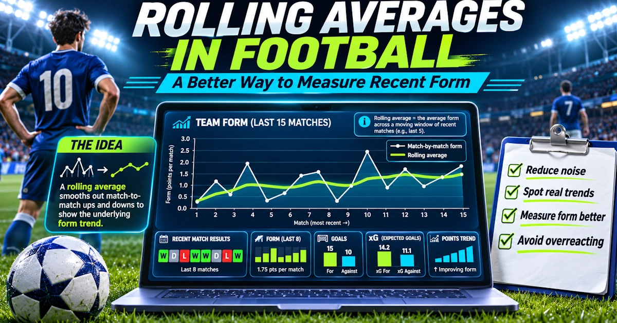
Rolling averages offer a better way to analyse recent form because they show how performance changes over time, rather than treating one fixed five-match block as the whole story. They are especially useful for:
Goals scored and Goals conceded
The goal is not to make football analysis more complicated. It is to make recent form less dependent on one unusual match.
What Is a Rolling Average?
A rolling average calculates the average of a statistic across a fixed number of recent matches and then updates after every new game. For example, imagine a team records these xG numbers:
Match 1: 1.1
Match 2: 1.4
Match 3: 1.8
Match 4: 1.6
Match 5: 2.0
Match 6: 2.2
A five-match rolling xG average after Match 5 would be (1.1 + 1.4 + 1.8 + 1.6 + 2.0) ÷ 5 = 1.58 xG. After Match 6, the oldest match drops out.
Now we calculate (1.4 + 1.8 + 1.6 + 2.0 + 2.2) ÷ 5 = 1.80 xG. The average has increased.
That tells us the team’s attacking performance may be improving.
Why Rolling Averages Are Better Than a Static Last-Five Number
The phrase “last five matches” usually gives you one snapshot. A rolling average gives you a sequence.
For example, a five-match rolling xG might look like this:
After Match 5: 1.25
After Match 6: 1.31
After Match 7: 1.45
After Match 8: 1.62
After Match 9: 1.71
Now you can see a trend. The team is not simply “in good form.”
Its underlying attacking output has been improving gradually. That is much more useful for football predictions.
Rolling Averages Reduce the Effect of One Strange Match
Suppose a team normally produces around 1.5 xG per match. Then it plays a weak opponent and records 4.1 xG.
If you only look at that match, the attack suddenly appears elite. A rolling average softens the effect.
Imagine the previous four xG numbers were 1.4, 1.6, 1.3, and 1.7. Add the 4.1, and the total is 10.1.
The five-match average is 2.02 xG. That is higher than normal, but it is nowhere near 4.1.
The rolling average recognises the strong performance without pretending it represents the team’s normal level.
Rolling Averages Are Particularly Useful for xG
Expected goals can fluctuate significantly from match to match. One game may contain a penalty, a red card, or an open final 20 minutes.
Another may be a slow 0-0. Looking at xG across several matches smooths out some of that noise.
Suppose a team’s last five xG values are 0.9, 1.1, 1.6, 1.8, and 2.0. The five-match average is 1.48.
But the sequence also tells us something important. The team has improved in each of its last four games.
A single average hides that trend, while a rolling series makes it visible.
Rolling xGA Can Reveal Defensive Decline
The same method works defensively. Suppose a team’s five-match rolling xGA moves like this: 0.85 → 0.92 → 1.10 → 1.29 → 1.47.
That is a clear warning sign. Maybe the final results still look good because the goalkeeper has been excellent.
But the defence is allowing better chances over time. If the next opponent is a strong attacking team, that deterioration becomes relevant for Over 2.5, BTTS, or Opponent Team Total.
This is one of the biggest strengths of rolling averages. They can reveal changes before those changes are obvious in the scoreboard.
Practical Example: Results Look Good, Rolling Numbers Do Not
Imagine Team A has 4 wins from its last 5 matches, which looks like very strong form. But its five-match rolling xG looks like 1.65, 1.58, 1.51, 1.43, and 1.32.
Its attacking output is declining. Meanwhile, actual goals remain high because finishing has been excellent.
The wins are real, but the rolling data suggests the attack may be becoming less dangerous. If the next opponent has a strong defence, blindly backing Team A because of the winning streak may be risky.
Practical Example: Poor Results, Improving Performance
Now imagine Team B has 1 win from its last 5, which looks like bad form. But its rolling xG moves: 1.05, 1.21, 1.39, 1.57, and 1.76.
Its rolling shots on target also rise: 3.1, 3.5, 4.0, 4.4, and 4.9. The results are poor, but the performances are improving.
If the bookmaker price becomes too negative because of the recent losses, this could create value.
Use More Than One Rolling Window
There is no perfect rolling-average length. Different windows answer different questions.
A useful approach is to compare a 3-match rolling average, a 5-match rolling average, and a 10-match rolling average. The three-match number reacts quickly, while the ten-match number is more stable.
Suppose a team’s xG averages are 3-match (1.95), 5-match (1.72), and 10-match (1.46). That suggests recent improvement.
Now suppose they are 3-match (1.05), 5-match (1.28), and 10-match (1.55). That suggests decline.
Comparing several windows gives more context than relying on only one.
Short Windows React Faster but Create More Noise
A three-match rolling average is sensitive. Imagine these xG values: 1.0, 1.1, and 3.2.
The three-match average is 1.77. One huge performance has a major impact.
That makes short windows useful for detecting quick changes, but they are also more vulnerable to random variation. For predictions, short rolling averages should normally be checked against longer ones.
Longer Windows Are More Stable but Slower
A ten-match average is harder to distort. One unusual match matters much less, but that stability creates another problem.
Suppose a team changes manager. The first five matches under the new coach may be completely different from the previous tactical system.
A ten-match rolling average still includes several matches under the old manager, so the statistic may react too slowly. This is why context remains essential.
Rolling Goals Can Be Useful, but xG Is Usually More Informative
Suppose a team’s rolling goals average rises: 1.2, 1.5, 1.8, and 2.1. That looks positive, but check xG too.
If rolling xG stays around 1.3, the team may simply be finishing unusually well. Now suppose both goals and xG rise together.
That is much stronger evidence of genuine improvement. Use actual goals to show outcomes, and use xG to test whether those outcomes are supported by chance creation.
Practical Example: Over 2.5 Prediction
Imagine the home team’s 5-match rolling xG is 1.4 → 1.6 → 1.8 → 1.9, and xGA is 1.2 → 1.4 → 1.5 → 1.6. The away team’s 5-match rolling xG is 1.3 → 1.4 → 1.5 → 1.7, and xGA is 1.4 → 1.5 → 1.7 → 1.8.
Both teams are creating more and conceding more. That combination can strengthen an Over 2.5 case.
The important part is not one high-scoring result. It is the direction of the trend.
Practical Example: Under 2.5 Prediction
Now imagine the home team’s rolling xG is 1.7 → 1.5 → 1.3 → 1.1. The away team’s rolling xG is 1.5 → 1.4 → 1.2 → 1.0.
Both attacks are declining, and at the same time, rolling xGA is improving. Possible interpretation: lower chance creation, better defensive organisation, and fewer open matches.
That can support an Under prediction if other factors agree.
Rolling Shots on Target Add Useful Confirmation
xG should not stand alone. Suppose rolling xG is rising, which is encouraging.
Now check rolling shots on target. For example, xG moves 1.2 → 1.4 → 1.6 → 1.8, while shots on target move 3.2 → 3.6 → 4.1 → 4.8.
Two independent measures are moving in the same direction. That increases confidence that the attack is genuinely improving.
If xG rises but shots on target collapse, investigate why.
Big Chances Can Be Added Too
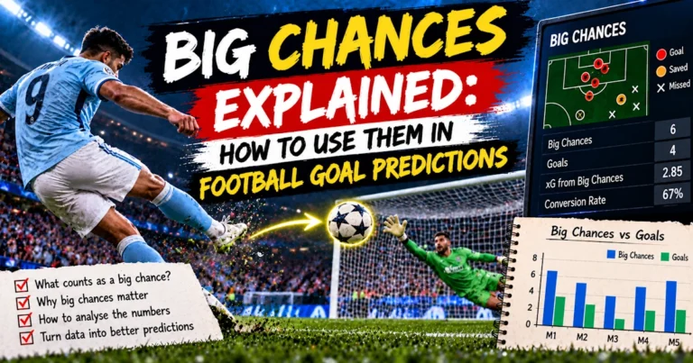
Rolling big chances can help identify whether improvement comes from genuine clear opportunities. For example, a five-match rolling big chances created looks like this: 1.1, 1.3, 1.6, 1.9, and 2.2.
That suggests a team is increasingly reaching dangerous areas. Now combine that with rising xG, and the trend becomes much more convincing.
Separate Home and Away Rolling Averages
This is especially important. Suppose a team’s overall rolling xG is 1.8, but home rolling xG is 2.1 and away rolling xG is 1.3.
The next match is away, so the overall figure may overstate its attacking potential. Where possible, compare the home team’s home rolling data against the away team’s away rolling data.
That gives a more relevant picture.
Adjust for Opponent Strength
Rolling averages can still be misleading if the schedule changes. Suppose a team records rising xG: 1.2, 1.5, 1.8, and 2.1.
Looks excellent, but those matches were against teams ranked 15th, 17th, 18th, and 16th. Now it faces the league leader.
The trend is real, but the opposition quality has been unusually favourable. Rolling averages reduce noise, but they do not automatically correct for schedule difficulty.
Manager Changes Can Break the Series
Suppose the rolling average uses eight matches, and a new manager arrives after Match 5. The next three matches show dramatically different tactics.
The eight-match average still mixes the old system and the new system. This can hide the tactical change.
In such cases, consider restarting your analysis from the coaching change or giving newer matches greater weight.
Injuries Can Change the Meaning of the Trend
Suppose a team’s rolling xG has risen to 1.9. But its main striker and creative midfielder are now injured.
That historical average may no longer represent the current lineup. Statistics describe the team that produced them.
If the personnel changes, your prediction should change too. Rolling averages are useful, but they are not immune to team news.
Red Cards Can Distort Rolling Numbers
Imagine one match produces 3.6 xG because the opponent played with ten men from the 20th minute. That match remains inside the rolling window for several games, and it can continue inflating the average.
Do not automatically remove unusual matches, but mark them mentally. Ask whether the conditions are likely to repeat.
Weighted Rolling Averages Can Be Even Better
A basic rolling average gives each match equal importance. A weighted rolling average gives more importance to recent games.
Suppose the last five xG values are 1.0, 1.2, 1.5, 1.8, and 2.1. Instead of treating every game equally, you might give the newest matches larger weights.
For example, oldest match (10%), next (15%), next (20%), next (25%), and newest (30%). The weighted average becomes more responsive to recent improvement, which can be useful when team performance is changing quickly.
But Avoid Making the Model Too Complicated
There is a danger here. More mathematics does not automatically create better predictions.
A complicated weighted model can give a false sense of precision. You do not need to calculate 1.684739 xG and pretend that number is exact.
The goal is simply to distinguish between improving, stable, and declining. A simple five-match rolling average often does the job perfectly well.
Rolling Averages Are Excellent for Charts
One of the best ways to use rolling averages is visually through statistical platforms like Opta Analyst or FBref. Imagine a chart with 5-match rolling xG and 5-match rolling xGA.
If xG rises while xGA falls, the team is improving at both ends. If xG falls and xGA rises, performance is deteriorating.
If both rise, games may be becoming more open. This can help identify goal-market trends quickly.
Look for Crossovers
A useful pattern occurs when rolling xG crosses rolling xGA. Suppose earlier xG was 1.2 and xGA was 1.6.
Later, xG is 1.7 and xGA is 1.3. The team has moved from being out-created to creating more than it concedes.
That may signal genuine improvement. But do not treat one crossover as a guaranteed turning point; confirm it with several matches.
Rolling Averages Can Help Find Market Overreaction
Suppose a team loses three straight. The betting market reacts, and its odds become longer.
But rolling performance shows xG stable around 1.7 and xGA stable around 1.1. The team may simply have suffered poor finishing and strong opposition goalkeeping.
The losing streak looks dramatic, but the rolling numbers do not. That can help identify situations where recent results are receiving too much attention.
The Opposite Can Happen After Winning Streaks
A team wins five straight, and its price becomes shorter. But rolling xG is falling: 1.8, 1.7, 1.5, 1.4, and 1.2.
Meanwhile, goals remain high. That can indicate the market is reacting to results while underlying performance is weakening.
Rolling averages help you notice the gap.
Rolling Average Prediction Checklist
Before using a rolling trend, check:
Window length
xG, xGA, and goals
Shots on target and big chances
Home-away split and opponent quality
Red cards and penalties
Manager changes, injuries, and rotation
Whether several metrics agree
Whether the market has reacted to recent results
A rolling average is most powerful when the trend makes football sense.
Frequently Asked Questions
What is a rolling average in football? It is the average of a statistic across a fixed number of recent matches, recalculated after every new game. For example, a five-match rolling xG average always uses the most recent five matches.
Is a five-match rolling average better than simple last-five form? Usually it provides more information because you can track how the average changes over time rather than looking at only one snapshot.
Which statistics work best with rolling averages? xG, xGA, goals, shots on target and big chances are particularly useful.
Should I use three, five or ten matches? There is no perfect window. Three matches reacts quickly but is noisy, five provides a useful balance, and ten is more stable but slower to detect change.
Can rolling averages predict goals? They can help identify improving or declining attacking and defensive trends, but they should still be combined with opponent strength, lineups, venue and the available odds.
Final Thoughts
Recent form matters. The problem is that the standard last-five table can make it look more precise than it really is.
One large win can distort the numbers, and a difficult run of opponents can make a good team look poor. A lucky finishing streak can make an average attack look elite.
Rolling averages give you a better way to see what is actually changing. Instead of asking: “What happened in the last five matches?”, you can ask: “Is performance improving, declining or remaining stable over time?”
That is a much better question for football predictions. Use rolling xG to follow attacking quality, and use rolling xGA to monitor defensive performance.
Add shots on target and big chances to confirm the pattern. Then adjust for opponent strength, venue, injuries, rotation and tactical changes.
The biggest benefit of rolling averages is not that they create a perfect prediction model. They help reduce the influence of short-term noise.
And in a sport where one penalty, red card or lucky finish can completely change a match, reducing noise is often one of the most valuable things you can do.
Responsible betting: Rolling averages can help identify football trends but cannot guarantee future results. Combine them with current team information and larger samples, compare your estimated probability with the available odds, keep stakes controlled and never bet money you cannot afford to lose.